STA130: Lecture_9

Classification (Decision) Trees §

Anatomy of a classification tree §

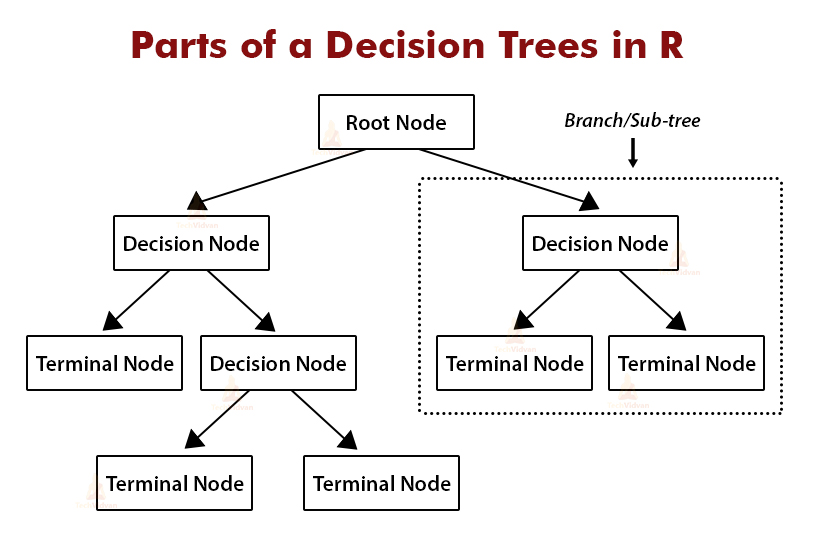
• Decision Tree - flowchart-like diagram that shows the various outcomes from a serious of decisions. Advantage is its easy to follow and understand
• Root node - the starting point of the tree (first parent node), same functionality with terminal (leaf) nodes.
• Leaf nodes - child nodes, contain a question or criteria to be answered, the answer splits into exactly two child nodes
• Terminal nodes - the node containing the prediction results of the decision tree.

Build a Simple Tree §

Code to build the tree using R §

library(rpart)  # Package which includes the rpart() function, used to build trees
library(partykit)  # Package which includes as.party(), used to visualize trees

tree <- rpart(<y> ~ <x_1> + <x_2>, data = <dataset>)
plot(as.party(tree), gp=gpar(cex=1), type="simple")  # gp is for visual adjusting

Predicting which people have trouble sleeping using Decision Tree in R §

• Using the sample of 2,500 individual’s survey in the US between 2009 and 2012 (NHANES)
• SleepTrouble as response variable; SleepHrsNight and DaysPhysHlthBad as predictors

Geometric interpretation §

• Extended decision tree visual

  plot(as.party(tree), type="extended")

  • (produced by the code above)
• This is a “scattered plot”
  • The vertical line shows the split of the first predictor, while the horizontal lines shows the split of the second predictor
  • (Code is not shown [not important here])

How to fit a Tree (mostly done by R) §

Goal: each terminal (leaf) node to be as pure as possible; and the tree as simple as possible

1. A response variable ($y$ what the tree want to predict)
2. A set of candidate predictors ($x_i,i=1,\dots ,M$)
3. A set of binary questions (ex. $x_i\ge 25$) [Need categorical response and binary splits, binary splits are based on predictors:]
   • Numerical predictors can be split based on the range (ex. $x_i\ge 25$)
   • Categorical predictors can be split based on the categories (choose 2 if there is more)
4. A method to evaluate if a spits
   • [A “good” split is one that makes its child node as pure as possible]
     • Pure node - if the node only contains observations from one class
     • Impure node - if the node contains an equal mix of all the classes (50% each category)
     • Measures of impurity
       • $Gini(t)=1-(w_i(t){)}^2+(w_2(t){)}^2$
       • $Entropgy(t)=-w_1(t){\log }_2(w_1(t))+w_2(t){\log }_2(w_2(t))$
   • [The “best” split is the one with the biggest decrease in impurity $\Delta I$]
     • For each candidate split, calculate the decrease in impurity as $\Delta I$ (measures the pure of the two child, compared tot he parent’s pure)
     • After looking at each of the potential predictor and each possible splits, choose the best
5. A rule to decide when to stop splitting
   • Simple rule: set a threshold $\beta >0$
   • If none of the splits of a node makes the tree at least $\beta$-units pure, then don’t split further
6. A way to make a prediction for each terminal node

Evaluating the prediction accuracy of a tree (categorical predictor) §

• Accuracy rate - how close the predictions are to the true values, on average

Accuracy = \frac{\text{# of correct predictors}}{\text{total # of predictions}}

• Confusion matrix - a table with one row for each predicted class and one column for each tree class

  	Actually positive	Actually negative
  Predict positive	True positives (TP)	False positives (FP)
  Predict negative	False negative (FN)	True negatives (TN)

• For a binary response, there are 2 types of errors [incorrect, want rate to close to 0]

  • False positive error - predict (+) by D.T. but actually is (-) [inconvenience]
  • False negative error - predict (-) by D.T. but actually is (+) [might cause negative impact]

• 2 important properties of the prediction model [correct, want close to 1]

  • Sensitivity - proportion of actual (+) correctly predicted as (+)
  • Specificity - proportion of actual (-) correctly predicted as (-)

• Another way to define the accuracy rate:

Accuracy = \frac{\text{# True positives}~ + ~\text{# True negatives}}{\text{Total # of predictions}}

Strategies for assessing the prediction accuracy of a tree §

1. Randomly divide data into “training” and “testing” datasets (80% for training, and 20% for testing)
2. Fit the tree based on the training data only
3. Run the test through the fitted tree to make predictions, and construct a confusion matrix to see how many are correctly/incorrectly classified

Example with the NHANES dataset §

NHANES <- NHANES %>% rowid_to_column()  # add a new ID to columm

# Find n, the total number of observations
n <- nrow(NHANES)

# Set training and testing data
set.seed(1002)
train_ids <- sample(1:n, size= round(0.8*n))

train <- NHANES %>% filter(rowid %in% train_ids)
test <- NHANES %>% filter(!(rowid %in% train_ids))

# Fitting the data
tree <- rpart(SleepTrouble ~ SleepHrsNight + DayPhysHlthBad, data=train)
plot(as.party(tree), type="simple", gp=gpar(cex=0.8))

# Constructing confusion matrix
tree_pred <- predict(tree, newdata=test, type="class")
table(tree_pred, test$SleepTrouble)

##
##	tree_pred	No		Yes
##		   No	339		133
##		  Yes	9		19

• Accuracy = $(339+19)/(339+133+9+19)=358/500=0.716$
• False positive rate = $9/(339+9)=9/348=0.026$
• False negative rate = $133/(133+19)=133/152=0.875$ (not so good)

Comparing different trees §

1. Use rpart() to specify different sets of candidate predictors to predict the same response
2. (optional) Plot all trees’ visual out with as.party()
3. Constructing confusion matrices for all trees (based on the testing data)
4. Constructing confusion matrices for all trees (based on the training data)
5. Combine the 2 tables above, use it to compare the trees
   • Understand the priority between accuracy/sensitivity/specificity for the given problem
     • Ideally all of these should be high, but may have to prioritize one over another
   • Ideally, prefer the tree to be less complex (less risk of overhitting, more interpretable)

Response variable has more than 2 levels §

• The classification tree method still works
• The confusion matrix is a $m\times m$ matrix, where $m$ is the number of levels of the response
• Sensitivity and specificity does not apply anymore
• Careful for the different types of possible errors

Limitations for training and testing approach §

• The accuracy of trees (or RMSE for linear regression models) depends on which observations are in the training/testing sets, which are determined at random
• Only a single subset of the observations are used to build(or fit) the prediction model
  • Statistical methods perform better when more data is used to fit them
  • This approach may make the error rate look a bit worse than it would be if all of the data were used to fit the model (without splitting the training and testing set)