STA130: Lecture_2

Variable types and distributions §

Variable Types §

• Quantitative Data (numerical values)

  • ==The differences of numbers are meaningful== (numbers are not arbitrary labels)
  • Continuous variables - any possible value within a certain range
  • Discrete variables - some values within a certain range

• Categorical Data (values represent categories)

  • Nominal variables - the categories don’t have a particular order
    • Binary - only 2 mutually exclusive outcomes (a special type fo nominal variable)
  • Ordinal variables - the categories are ordered in a particular way

Variable Distribution §

• What value does the variable take (the possible range of the values)
• How often does the variable takes from each range of values (possibility of the outcome)
• 3 key elements: shape, centre, spread

---

Distribution of quantitative variables §

Histograms §

• Height of each bar is the frequency in which variable appear in the corresponding bin

• The horizontal axis is numerical and has no gaps in between (represent bins)

• The vertical axis represents the frequency in which the values fall under each bin

• Use geom_histogram() to create a histogram in R

  ggplot(data = name_of_dataset, aes(x = name_of_visualize_variable)) +
  	goem_histogram(color="black",  # color of the outline
                    fill="grey",   # color of the fill
                  bins=30) +     # number of bins for the x axis (divide by 30 here)
  	labs(x = "label of the x-axis")

• Have to decide a “just right” number of bin in which accurately highlights the interesting features of the distribution, but does but over-represented it

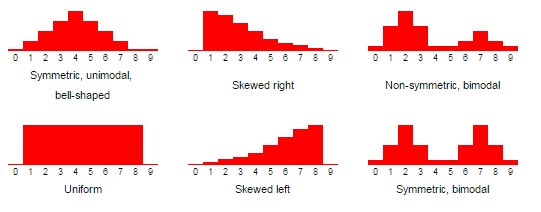
Shape - the overall pattern fo the values §

• Skewness to the direction of the longer tail (Symmetric vs. Left-skewed vs. Right-skewed)

• The number of modes or modality of the graph (Unimodal vs. Bimodal vs. Multimodal vs. Uniform)

  

Centre - describes a “typical” value fo the variable §

• Mean - the “average” number of the dataset, shows the centre

  $\bar{x}=\frac{x_1+x_2+\cdots +x_n}{n}=\frac{1}{n}{\sum }_{i=1}^n{x}_i$

  • Calculating $n$(adding the total height of the bars) and ${\sum }_{}{x}_i$(adding the height times the middle value) to get a mean estimation [be careful of how each are represented in the graphs]

• Median - best measure of centre to use in a skewed distribution

  • Half of the values are smaller than the median; Half of the values are larger than the median
  • Estimate by rank/sort values (by getting $n/2$’s value for the graph)

• Modality - mode, the most commonly observed value in a set of data

• No measure is superior, each provides different information

Spread - concentration of the values §

Focus is not calculation, but understanding and know that each represents

• Variance - roughly the average squared distance between the values and their mean

  $s^2=\frac{(x_1-\bar{x}{)}^2\cdots +(x_n-\bar{x}{)}^2}{n-1}=\frac{1}{n-1}{\sum }_{i=1}^n(x_i-\bar{x}{)}^2$

• Standard deviation (sd) - squared root of the variance $s=\sqrt{s^2}$

  • Its a popular measure of spread because it measures in the same units but is easier to interpret
  

Boxplot - visualizing a summary of centre/spread for numerical distributions §

• Summarizes the distribution of quantitative variables using 5 stats, while also plotting outliers if any

  1. Line in the middle of the box: median ($Q2$)
  2. Edges of the box
     • Lower edge: first quartile ($Q_1$) - 25% of the data is smaller than this number
     • Upper edge: third quartile ($Q_3$) - 75% of the data is smaller than the number

3. Length of the box: inter-quartile range (IQR), from $Q_3-Q_1$ which shows the range in which 50% of the values lie
4. Whiskers on the box extend to the extreme values that is within $1.5$ X IQR of the box
5. Points beyond the whiskers: outliers - unusual values that worths investigations

• Each x value is a single boxplot, while the y value is the accumulated value data

• Use geom_boxplot() to create boxplot in R

  • aes stands for aesthetic

  ggplot(data = name_of_dataset, aes(x = categorical_variable, y = visual_variables)) + 
                                   # x = "" if only want one boxplot
  	geom_boxplot(color="black", fill="grey") + 
  	labs(y = "label_for_y_axis", 
         	 x = "lavel_for_x_axis")  # don't need this line if (x = "")

---

Distribution of categorical variables §

Barplots §

• Used to visualize the distribution of a categorical variable with 2 or more categories

• One bar for each category, orders and widths are arbitrary (widths should all be the same)

• The height counts the frequency in which the variables appears in the corresponding category

• There is a gap between each bar with the same width

• Shape and centre not meaningful because the order of categories are arbitrary

  • One exception is original variables

• Use geom_bar() to create a barplot

  ggplot(data = name_of_dataset, aes(x = name_of_varaible)) + 
  	geom_bar(color="black", fill="grey") + 
  	labs(x = "label for the x axis") # + 
  	# coord_flip()  # add this line ONLY IF want the graph to be vertical

Distribution of categorical variable §

• Most common and least common categories (order of frequency)
• Magnification of the frequency between each categories